CUDA Studylog 2 - Matrix Multiplication and 2D Grid Organization
In our previous post, we explored the basics of CUDA programming through a simple RGB to grayscale conversion in 1D grid and block computation. Now, let’s look into CUDA’s 2D grid structure by tackling something more fundamental to machine learning: matrix multiplication.
Understanding Matrix Multiplication
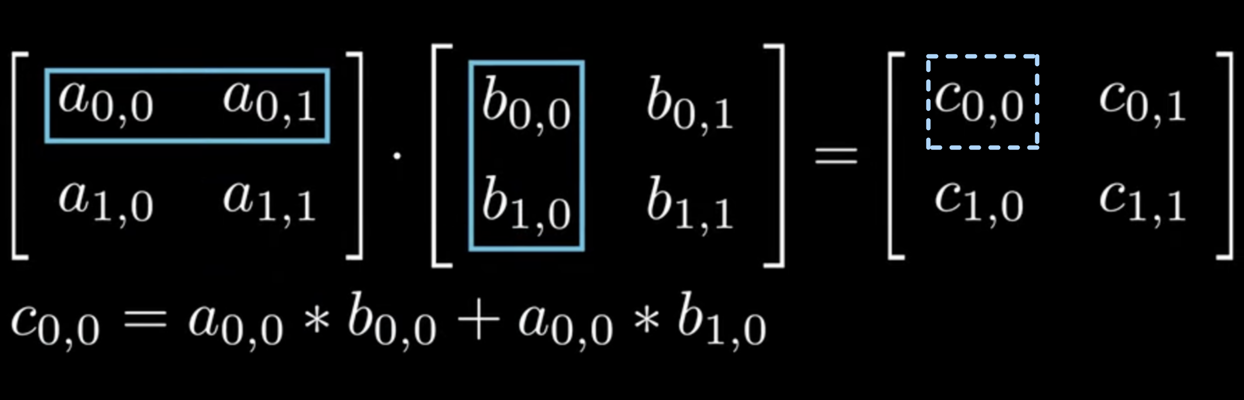
Let’s start by refreshing our understanding of matrix multiplication. For matrices A (M×K) and B (K×N), the result C (M×N) is computed as shown in Figure 1:
In traditional CPU code, matrix multiplication would look like this:
# Python implementation
def matmul(A, B):
    M, K = A.shape
    K, N = B.shape
    C = np.zeros((M, N))

    for i in range(M):
        for j in range(N):
            for k in range(K):
                C[i,j] += A[i,k] * B[k,j]
    return C
Mapping Matrix Multiplication to CUDA Threads
When implementing matrix multiplication in CUDA, we need to think about how to map our computation to GPU threads. The key principle, as discussed in our previous post, is to think in terms of output elements. Each thread will be responsible for computing one element of the output matrix C.

Implementation Approaches
1. Using 1D Grid (The Simple Approach)
Our first instinct might be to flatten the 2D output matrix into a 1D array, similar to our grayscale conversion example. Here’s how that would look:
inline unsigned int cdiv(unsigned int a, unsigned int b) { return (a + b - 1) / b;}

__global__ void matmul_1d_kernel(float* A, float* B, float* C, int M, int N, int K) {
    int idx = blockIdx.x * blockDim.x + threadIdx.x;
    if (idx >= M * N) return;

    int row = idx / N; // row index of the output matrix
    int col = idx % N; // column index of the output matrix

    float sum = 0.0f;
    for (int k = 0; k < K; k++) {
        sum += A[row * K + k] * B[k * N + col];
    }
    C[idx] = sum;
}
Note: All code snippets in this post are available in the following notebook..
However, this 1D approach has several limitations:
- It makes our code less intuitive and harder to reason about
- It can lead to less efficient memory access patterns
- It doesn’t take advantage of CUDA’s built-in support for multidimensional data
Understanding CUDA’s dim3 Type
To address these limitations, we need to understand how CUDA enables multidimensional computation through the dim3 type. The dim3 struct is a fundamental CUDA type that helps organize threads in up to three dimensions.
When launching a CUDA kernel, we use the <<<grid>>> syntax to specify grid and block dimensions. CUDA provides two ways to specify these dimensions:
- Simple integers (for 1D organization):
int threadsPerBlock = 256; // Number of threads in each block int numBlocks = cdiv(N*M, threadsPerBlock); // Number of blocks needed kernel<<<numBlocks, threadsPerBlock>>>(args...); - dim3 structs (for 2D/3D organization):
// For 2D organization (like our matrix multiplication):
dim3 threadsPerBlock(16, 16);    // 16x16 threads per block (z=1 by default)
dim3 numBlocks(
    cdiv(N, threadsPerBlock.x),  // Number of blocks in x direction
    cdiv(M, threadsPerBlock.y)   // Number of blocks in y direction
);
kernel<<<numBlocks, threadsPerBlock>>>(args...);

// For 3D organization (useful in volume processing, 3D convolutions):
dim3 threadsPerBlock(8, 8, 8);   // 8x8x8 threads per block
dim3 numBlocks(
    cdiv(width, threadsPerBlock.x),
    cdiv(height, threadsPerBlock.y),
    cdiv(depth, threadsPerBlock.z)
);
Inside the kernel, we can access these dimensions and calculate global indices:
// For 1D:
int idx = blockIdx.x * blockDim.x + threadIdx.x;

// For 2D:
int row = blockIdx.y * blockDim.y + threadIdx.y;
int col = blockIdx.x * blockDim.x + threadIdx.x;

// For 3D:
int x = blockIdx.x * blockDim.x + threadIdx.x;
int y = blockIdx.y * blockDim.y + threadIdx.y;
int z = blockIdx.z * blockDim.z + threadIdx.z;
Note that
blockIdxandthreadIdxare built-in variables in CUDA that store the block and thread indices respectively. The grid dimensions defined inside<<<>>>are passed as follows: the second parameter (block size) becomes available asblockDiminside the kernel, while the first parameter (grid size) determines how many blocks will be launched.blockDimis particularly important as it’s used to calculate global thread positions from local indices.
2. Using 2D Grid (The Natural Approach)
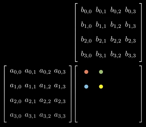
Now that we understand how to organize threads in multiple dimensions using dim3, let’s see how we can use it to implement matrix multiplication in a more natural way. CUDA’s 2D grid structure aligns perfectly with our matrix computation:
The 2D grid organization provides several benefits:
- More intuitive mapping between threads and matrix elements
- Better alignment with matrix memory layout
-
Potential for optimized memory access patterns
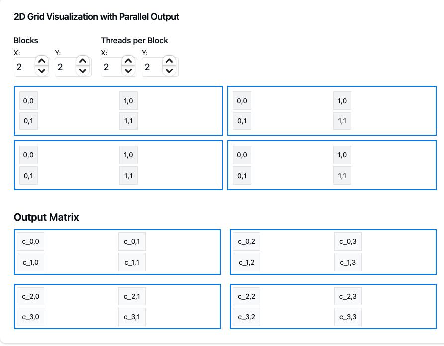
- Output Matrix Mapping:
- Each small cell represents one thread
- 2×2 blue squares represent thread blocks
- The entire grid covers the output matrix C
- Thread/Block Indexing:
- Global thread position:
int row = blockIdx.y * blockDim.y + threadIdx.y; // Global row in C int col = blockIdx.x * blockDim.x + threadIdx.x; // Global column in C - Each thread computes one element C[row,col]
- Block dimensions chosen as 2×2.
- Global thread position:
- Grid Size Calculation:
- Must cover entire output matrix
- Uses ceiling division to handle non-perfect divisions:
dim3 threadsPerBlock(16, 16);  // 256 threads per block
dim3 numBlocks(
   cdiv(N, threadsPerBlock.x)  // Ceil(N/16)
   cdiv(M, threadsPerBlock.y)   // Ceil(M/16)
);
__global__ void matmul_naive(float* A, float* B, float* C, int M, int N, int K) {
    // Global thread indices map directly to matrix coordinates
    int row = blockIdx.y * blockDim.y + threadIdx.y;  // y component for rows
    int col = blockIdx.x * blockDim.x + threadIdx.x;  // x component for columns

    if (row < M && col < N) {
        // ... computation ...
    }
}
This organization naturally extends to our tiled implementation where each block processes a 16x16 tile of the output matrix.
Naive CUDA Implementation
Let’s start with a straightforward CUDA implementation. Each thread will compute one element of the output matrix. Here’s our naive implementation using 2D grid organization:
__global__ void matmul_naive(float* A, float* B, float* C, int M, int N, int K) {
    int row = blockIdx.y * blockDim.y + threadIdx.y;
    int col = blockIdx.x * blockDim.x + threadIdx.x;

    if (row < M && col < N) {
        float sum = 0.0f;
        for (int k = 0; k < K; k++) {
            sum += A[row * K + k] * B[k * N + col];
        }
        C[row * N + col] = sum;
    }
}
To launch this kernel:
dim3 threadsPerBlock(16, 16);  // 256 threads per block
dim3 numBlocks(
    cdiv(N, threadsPerBlock.x),  // Ceil(N/16)
    cdiv(M, threadsPerBlock.y)   // Ceil(M/16)
);

matmul_naive<<<numBlocks, threadsPerBlock>>>(A, B, C, M, N, K);
Performance Considerations and Next Steps
To understand where we stand with our implementation, let’s compare it with PyTorch’s highly optimized matrix multiplication:
| Implementation | Time (ms) | Notes |
|---|---|---|
| Our Naive CUDA | 6.0 | Basic 2D grid implementation |
| PyTorch matmul | 2.0 | Highly optimized with tiling and memory coalescing |
As we can see, our implementation, while functional, is about 3x slower than PyTorch’s optimized version. This gap exists because our current implementation has several performance limitations:
- Memory Access Pattern: Each thread needs to read entire rows of A and columns of B from global memory, resulting in non-coalesced memory access.
- Memory Bandwidth: We’re repeatedly accessing the same data from global memory, which is expensive.
- Computation to Memory Access Ratio: The current implementation performs too many memory operations compared to compute operations.
In our next post, we’ll explore how to optimize this implementation using shared memory tiling and other advanced techniques to bridge this performance gap. We’ll see how techniques like memory coalescing, shared memory usage, and other tricks can help us get closer to PyTorch’s performance.
Stay tuned to learn how we can transform this naive implementation into a high-performance matrix multiplication kernel!

Leave a comment