Lightweight Guide to understanding GRPO and RL principles

Background & Motivation

This is a mini blog about understanding the GRPO (Group Relative Policy Optimization) training workflow. This is a missing piece I wanted to read before implementing my own workflow.

Most content creators assume the reader to be aware of GRPO’s predecessors like DPO/PPO and then talk about GRPO, which obviously shoos away the people with no prior RL knowledge. If you haven’t touched RL/Reinforcement Learning before, you are at the right place.

---

What is GRPO?

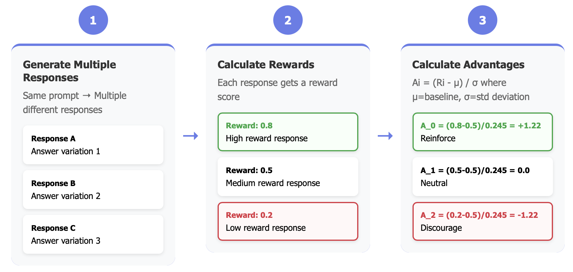
GRPO works on the FAFO principle - Fool Around and Find Out. Here’s a brief overview of how it works: it generates multiple responses to the same prompt, calculates advantages for each response, and then teaches the model to favor responses with higher advantages and push back responses with lesser advantages.

Figure 1: GRPO Training Workflow Overview

Why Advantages?

Although reward is already signalling if a specific response is better, you want to know how better is the current response compared to other responses for the same query. This is where advantages come in. Advantage is calculated by normalizing the rewards with mean and standard deviation.

The core GRPO objective function is:

Figure 2: GRPO Objective Function

Alright, it’s big and scary. Let’s focus on the atomic unit from above i.e

\[\mathcal{L}_{GRPO} = \frac{1}{G} \sum_{i=1}^{G} \frac{1}{|o_i|} \sum_{t=1}^{|o_i|} \pi_\theta(o_{i,t}|q, o_{i,<t}) \hat{A}_{i,t}\]

Now, let’s convert this to code.

for each_generated_answer_G in generated_answers: # G in the equation
    advantage = calculate_advantage(each_generated_answer_G)
    for each_token_o_i in each_generated _answer: # |o_i| in the equation
        token_loss = pi_theta(each_token_o_i) * advantage

    loss_of_each_answer = sum(tokens_loss_in_answer) / len(each_generated_answer )

final_loss = sum(loss_of_all_answers) / len (generated_answers) # G in the equation

Here, the pi_theta simply refers to the log probabilities of the token \(o_{i,t}\) given the query $q$ and the previous tokens $o_{i,<t}$.

From the figure 3 below (same as figure 2), we can see that the advantage is calculated at sequence level or answer level. So, for each token, the loss is calculated as the product of the log probability of the token $o_{i,t}$ and the advantage ($\hat{A}_{i,t}$):

\[token\_loss = \pi_\theta(o_{i,t}|q, o_{i,<t}) \times \hat{A}_{i,t}\]

Figure 3: GRPO Workflow Overview

Easy! We just implemented the atomic unit of GRPO loss calculation, which is just a two-nested for loop over the token losses of each answer.

\[\mathcal{L}_{GRPO} = \frac{1}{G} \sum_{i=1}^{G} \frac{1}{|o_i|} \sum_{t=1}^{|o_i|} token\_loss\]

where token_loss is the loss of each token in the answer i.e

\[token\_loss = \pi_\theta(o_{i,t}|q, o_{i,<t}) \times \hat{A}_{i,t}\]

The Hidden Challenge: Training on Stale Data

So far, we’ve looked at the basic GRPO loss calculation. But here’s what actually happens during GRPO training that creates an interesting challenge:

1. Generate a batch of answers using your current model (let’s say 4 answers per prompt)
2. Calculate advantages for these answers (which one is better/worse)
3. Train on this SAME batch for multiple gradient steps (e.g., 10 steps)

This is problematic because we generate answers ONCE, but train on them MULTIPLE times. This is great for efficiency, but it creates a subtle problem.

Why This Is a Problem?

Think about it: By gradient step 10, your model has changed from all the training. But we’re still using answers that were generated by the model from step 1!

It’s like practicing basketball shots based on a video of yourself from last week. You’ve improved since then, so the video doesn’t represent your current form anymore. This mismatch is called distribution shift or off-policy training.

Here’s what goes wrong if we ignore this:

# Generate answers with initial model
answers = model.generate(prompt)  # Model at step 0
advantages = calculate_advantages(answers)

# Train for multiple steps on the SAME answers
for step in range(10):
    log_probs = model.get_log_probs(answers)  # Model at step 1, 2, ... 10
    loss = log_probs * advantages
    model.update(loss)
    # By step 10, we're calculating gradients as if the current model
    # generated these answers, but it didn't! The step-0 model did!

This leads to increasingly biased gradients and unstable training. Your model might even “unlearn” good behaviors because it’s confused about where the data came from or why are the gradient updates not working as expected as answers remain constant from step 1 to step 10.

The Solution: Importance Sampling

This is where $\pi_{\theta_{old}}$ comes to the rescue. We keep track of the log probabilities from the model that ACTUALLY generated the answers (the “old” model), and use them to correct our loss calculation:

\[token\_loss = \frac{\pi_\theta(o_{i,t}|q, o_{i,<t})}{\pi_{\theta_{old}}(o_{i,t}|q, o_{i,<t})} \times \hat{A}_{i,t}\]

This ratio $\frac{\pi_\theta}{\pi_{\theta_{old}}}$ is called the importance sampling ratio. It tells us:

• Ratio > 1: Current model likes this token MORE than the old model did → amplify the gradient
• Ratio < 1: Current model likes this token LESS than the old model did → reduce the gradient
• Ratio = 1: Both models agree → gradient stays the same

In code:

# Generate answers ONCE with initial model
answers = old_model.generate(prompt)
old_log_probs = old_model.get_log_probs(answers)  # Store these!
advantages = calculate_advantages(answers)

# Now we can safely train for multiple steps
for step in range(10):
    current_log_probs = model.get_log_probs(answers)
    
    # The magic correction factor
    importance_ratio = exp(current_log_probs - old_log_probs)
    
    # Corrected loss that accounts for distribution shift
    loss = importance_ratio * advantages
    model.update(loss)

This correction ensures our gradients remain mathematically valid even though we’re training on “stale” data. It’s like adjusting your basketball practice to account for how much you’ve improved since the video was taken.

Adding Safety Rails: The Clipping Mechanism

But what if this importance ratio becomes extreme? Imagine the current model REALLY disagrees with the old model (ratio = 100 or 0.01). This could cause training to explode or collapse.

GRPO adds a safety mechanism: clip the ratio to stay within reasonable bounds:

\[ratio_{clipped} = \text{clip}(ratio, 1-\varepsilon, 1+\varepsilon)\]

With ε = 0.2 (typical value), the ratio can only vary between 0.8 and 1.2. This prevents any single update from being too aggressive, even if the models strongly disagree.

The full GRPO objective with clipping becomes:

\[\mathcal{L}_{GRPO} = \frac{1}{G} \sum_{i=1}^{G} \frac{1}{|o_i|} \sum_{t=1}^{|o_i|} \min\left(ratio_{i,t} \times \hat{A}_{i,t}, \text{clip}(ratio_{i,t}, 1-\varepsilon, 1+\varepsilon) \times \hat{A}_{i,t}\right)\]

The clipping is a conservative approach to prioritize stable training over perfect gradient correction.

# With clipping for safety
importance_ratio = exp(current_log_probs - old_log_probs)
clipped_ratio = torch.clip(importance_ratio, 0.8, 1.2)  # ε = 0.2

# Take the minimum of clipped and unclipped objectives
loss_unclipped = importance_ratio * advantages
loss_clipped = clipped_ratio * advantages
loss = torch.min(loss_unclipped, loss_clipped)

Why Not Just Generate New Data Every Step?

YYou might wonder: why go through all this complexity with importance sampling and clipping? Why not just generate fresh answers for every gradient step?

This touches on a fundamental concept in reinforcement learning: on-policy vs off-policy training.

On-Policy Training (The “Ideal” Approach)

In on-policy training, you generate new data from your current model for every single gradient update:

for step in range(training_steps):
    # Generate fresh data with current model
    answers = current_model.generate(prompt)
    advantages = calculate_advantages(answers)
    log_probs = current_model.get_log_probs(answers)
    
    # Simple, clean loss calculation
    loss = log_probs * advantages
    current_model.update(loss)

This is much simpler and mathematically “pure” - your gradients are always calculated with respect to data that your current model actually produced. No distribution shift, no stale data problems.

Off-Policy Training (The “Economic” Approach)

This is what we saw earlier. In off-policy training, you reuse data that was generated by an older version of your model:

# Generate once with current model
answers = current_model.generate(prompt)
old_log_probs = current_model.get_log_probs(answers)
advantages = calculate_advantages(answers)

for step in range(10):  # Reuse same data for multiple steps
    new_log_probs = current_model.get_log_probs(answers)
    
    # Need importance sampling to correct for staleness
    importance_ratio = exp(new_log_probs - old_log_probs)
    loss = importance_ratio * advantages
    current_model.update(loss)

-	On-policy	Off-policy
Pros	• Mathematically cleaner (no correction factors needed) • Always training on “fresh” data from current policy • Gradients are exactly what you’d expect	• Sample efficient - reuse expensive generations multiple times • Much faster in practice (10x fewer generations needed) • Better compute utilization
Cons	• Extremely expensive! Generating LLM responses requires full forward passes with sampling • Wastes compute - you throw away each batch after one gradient step • Slower convergence in wall-clock time	• Requires complex corrections (importance sampling) • Risk of instability if model changes too much • Gradients become approximations rather than exact

Interesting Developments in the field

1. KL Divergence disappears

Notice that I didn’t cover the KL divergence term in the objective function. This is because latest research proved that it is not necessary to use KL divergence in the objective function.

If you look at recent GRPO implementations, you’ll notice something interesting: everyone sets β = 0, effectively removing the KL divergence term entirely! It turns out the clipping mechanism we discussed already prevents the model from changing too drastically. Citing Qingfeng’s blog post, “the clipped objective is designed as a replacement of constraint policy optimization in form of the KL divergence term. Thus, adding a KL divergence term is not necessary theoretically”

2. Why GRPO/RL Forgets Less than SFT?

The paper [“RL’s Razor” (Shenfeld et al., 2025)(https://arxiv.org/abs/2509.04259)] show that RL fine-tuning, especially on-policy training, forgets less than SFT, even when both reach the same performance on new tasks. This is great if you are training on a new task and want to keep the original model’s performance on standard benchmarks.

3. Focus on the “forking tokens”

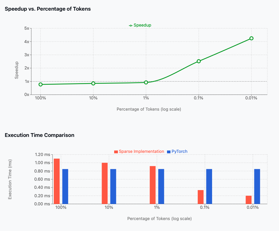
The paper “Beyond the 80/20 Rule” (Wang et al., 2025) discovered that only ~20% of tokens in reasoning sequences actually matter for learning & thinking exploration. These “forking tokens” at decision points drive nearly all performance gains.

Training on just these 20% of tokens not only maintains performance but actually improves it!

Conclusion

This is a lightweight guide to understanding GRPO and RL principles. I hope you found it helpful