Reducing the runtime from 2+ hours (on-GPU) to 8 mins in a recent project
Introduction
Prior to deploying a model to production data scientists must go through a rigorous process of code optimization which can be followed by upscaling using frameworks like Kubernetes/KubeFlow etc. I write this article/post from my experience of optimizing a raw code. Not necessarily correcting mistakes, but more to do with the identifying the deployment type and following good code practices.
For reader’s clarity, I categorized each mistake into a relevant concept. Concepts mentioned here are the ones we come across daily. What this blog emphasizes is not the concepts but identifying the need for such concepts and organizing your code to implement these concepts.
Context
The project aims to build a system that deidentifies critical information from healthcare documents. Specifically, the system has to process the uploaded PDF, run inference on multiple models and return a deidentified/redacted PDF with a few risk scores(domain-related: ignore).
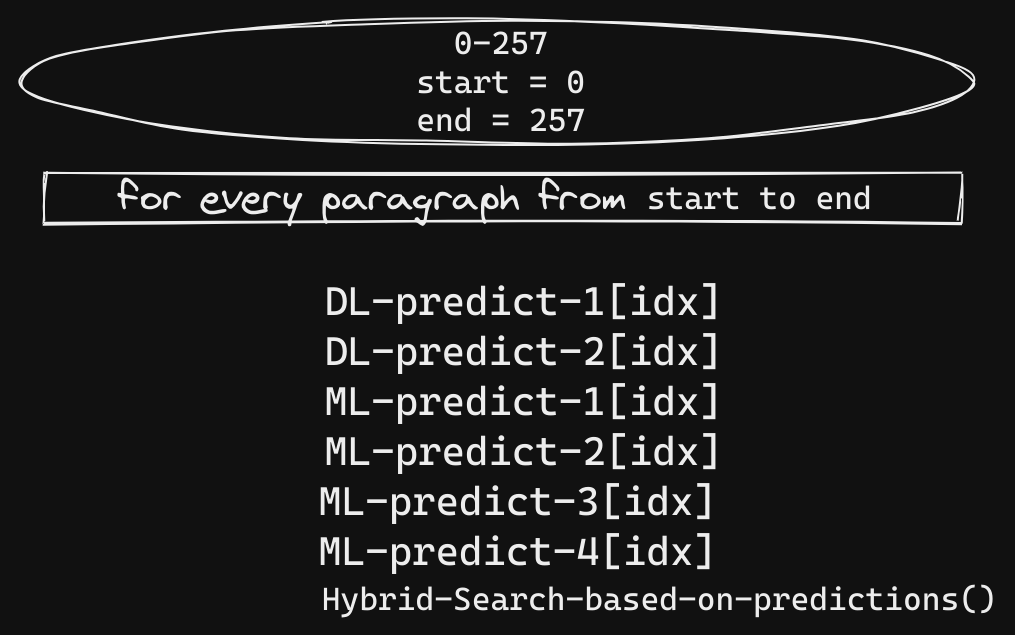
PDF upload & extraction time are discounted from the workflow mentioned below. Imagine that we start with the extracted paragraphs from PDF. So, project’s workflow can be approximated as below,
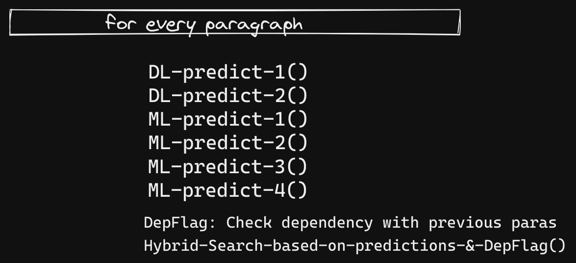
From the above pic, one could notice that there is a flag called DepFlag, which finds the relation b/w current and previous paragraphs. This, along with all the DL, ML models’ predictions of the para contribute to the main (necessary) step i.e Hybrid-Search. Hybrid-Search augments the current paragraph’s predictions with that of previous one’s and goes ahead in its search. This decision to augment is based on DepFlag since it informs if the current and previous paragraph come under a common heading.
Since there’s a clear dependency on the previous paragraph, the code has to run sequentially. Note the word Sequentially. This costed the team a running time of 2.5+ hours.
Product-design:
The system appears to look like Online Prediction since the user must wait for a de-identified PDF. As the average attention span of users is 8-seconds (Ref), it is not possible for the current system to perform all the operations (PDF extraction, Multiple model inference, Risk-Score calculations, De-identifying PDF) within 8 seconds.
So, the product design is changed to run the process in the background and notify the user once it’s done.
Before we start optimizing the code, we need to identify the inference type needed for our application.
Batch Prediction vs Online Prediction
Online Prediction is where predictions are generated as soon as the requests arrive.
Batch Prediction is where we process a high volume of samples that are pre-existing or accumulated over time. We perform the computation and store the results for later usage.
In Figure 1, we are performing Online Prediction, i.e ML-Predict, DL-Predict models are called for each paragraph and results are retrieved immediately.
Latency vs Throughput:
Latency is the time taken from receiving an input to returning the result whereas Throughput refers to the number of inputs processed per second.
In this code, throughput of the models is very less since we are processing only one sample at a time when it is possible to send multiple in parallel.
Using Batch Prediction to cut 1.25+ hours
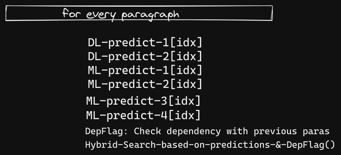
Since we already have the paragraphs stored, we can pivot the ML-Predict, DL-Predict function calls from Online Prediction to Batch Prediction in the following way,
1. Sequential predictions take time.
    For example, for processing 9000 instances,
        1. DL model took 27 minutes.
        2. ML model took 4.5 minutes.
2. Idea: Batch processing.
    a. Store all the paragraphs in a file.
    b. Make the models predict on them in batches(32,64,etc).
    c. Store results for all paras.
3. We can directly access the predictions.
4. Speed improvements:
    a. Batch Processing reduces the runtime
        1. For a DL model from 27 min into 3 min.
        2. For an ML model from 4min to 0.5 min.
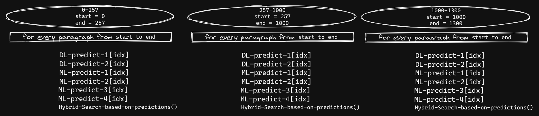
Shifting to Batch-Prediction didn’t change much in the main script (Figure 2 below) but we cut 1+ hours from the run-time. Also, prediction calls from DL-Predict & ML-Predict are quick now since results are pre-computed. This reduces the latency (since we are just indexing to get the results) and increases throughput (since we are processing many paras at once in the Batch Processing phase)
Parallel Processing
With Batch-Processing, we reduced the speed but code is still sequential. Hybrid-Search is still sequential. From context, it is clear that paragraphs that come under one heading need to be processed sequentially for Hybrid-Search. So, before the main script, we can create blobs(Blobs: group-of-paragraphs that fall under one heading).
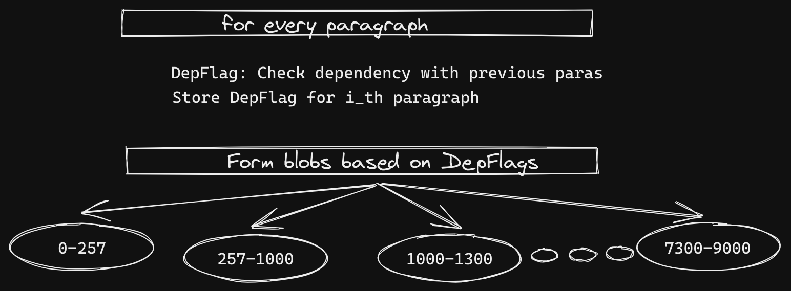
Now, we can run Hybrid-search on these blobs parallely.
This setup reduces/cuts-down the running time (post batch-processing) by 20+ min.
Involving SMEs - Subject Matter Experts
Rather than involving SMEs only at the labeling phase, it is a good practice to involve SME in every journey-step of the project. If it is costly to consult them at every stage, Business consultant can be a good substitute.
For example,
- To identify the author of a document, you need not run a Name-NER model on the entire document. Parsing the first few pages would do.
- Subject-ID & Patient-ID are essentially same. One can merge these two entities during training, etc.
As mentioned in the example, being-aware of the parsing-logic for a few entities saved us processing time (Around 10+ min).
Line-Profiling & Removing redundancies
While Line-Profiling isn’t new for engineers, I assume that it is for the Data-Scientists/Researchers. A typical Line-Profiler gives you a breakdown of your code in these aspects:
1. No.of hits for each line (#times each line is executed)
2. Running time of the line
3. Overall running time = (#hits) * (run-time-of-the-line)
4. Percentage contribution=> How much delay does the line
                             cause to the entire code.
With line-profiler, we are able to identify that a single dataframe operation (df.where) was taking 78% of the processing-time (post Batch processing & parsing-logic).
DataFrame operation
cols-of-interest = get 3 column-names out of 200-500+ columns
for each column in cols-of-interest,
    do a df.where in dataframe[column]
More columns vs less
Out of 200+ columns in the dataframe, only 10-14 columns were of interest. It was decided not to strip the unwanted columns since we are anyway accessing the dataframe through desired columns. However, we found that trimming the dataframe of unnecessary columns reduced running-time-load from 78% to 45%.
Much finer choices like Numpy vs Pandas, Column-access vs Row-access are addressed in Chip Huyen Chip Huyen’s CS329 lecture.
Conclusion
By identifying the type of inference, profiling, organizing and parallelizing the code, we are able to reduce the processing time. On a lighter note, I see the boundaries blurring between Data-Scientist and ML-Engineer. At this juncture, I believe that Data-Scientists must spend some time in learning engineering practices and writing production-ready code.
Note
Discussion around “GPU for inference” and “What/Why Hybrid-Search is used” are avoided to stick to the topic and also since they’re stakeholders decisions. All this optimization is done prior to the Growth/Scaling-up phase.

Leave a comment